Pre-Processing
OpenFOAM Case Structure
A case being simulated involves data for mesh, fields, properties, control parameters, etc. In OpenFOAM this data is stored in a set of files within a case directory rather than in a single case file, as in many other CFD packages. The case directory is given a suitably descriptive name, here exhaust_gas_recirculation. This folder contains the following subfolders and files:
├── 0
│   ├── alphat
│   ├── k
│   ├── nut
│   ├── omega
│   ├── p
│   ├── T
│   └── U
├── constant
│   ├── thermophysicalProperties
│   └── turbulenceProperties
├── system
│   ├── controlDict
│   ├── decomposeParDict
│   ├── fvSchemes
│   ├── fvSolution
│   └── meshDict
└── exhaust_gas_recirculation.obj

3 directories, 15 files
The relevant files for this tutorial case are:
0- This directory stores the initial values and boundary condition for each variables solved.constant- This directory contains files that are related to the physics of the problem, including the mesh and any physical properties that are required for the solver. In this case:thermophysicalPropertiesdefines the thermophysical properties of the fluid.turbulencePropertiesdefines, which turbulence model to use for the simulation.
system- This folder contains files related to how the simulation is to be solved:controlDictfor setting control parameters including start/end time, time step size and parameters for data output.decomposeParDictfor setting the number of processors in a parallel run.fvSchemesfor the discretization schemes used in the Finite Volume Method.fvSolutionfor the solver settings used in the Finite Volume Method.meshDictcontains the configuration for the automated meshing process.
Mesh Generation
The hexahedral-dominant, three-dimensional mesh is created automatically with the meshing utility cartesianMesh from a user provided surface geometry named `exhaust_gas_recirculation.obj, which is located in the case folder.
The exhaust gas recirculation pipe has a total length of \(360\,\text{mm}\) in \(x\)-direction with an air inlet diameter of \(40\,\text{mm}\) and an exhaust gas inlet with a diameter of \(20\,\text{mm}\). an initial channel height of \(H = 1\,\text{m}\) at the inlet and extends to \(4.7\,\text{m}\) towards the outlet. The maximum cell size is set to \(3\,\text{mm}\) resulting in about 13 cells across the large pipe diameter. Additionally, the walls have Five inflation layers with a thickness ratio of 1.3.
The resulting meshDict looks as follows:
// * * * * * * * * * * * * * * * * * * * * * * * * * * * * * * * * * * * * * //

surfaceFile "exhaust_gas_recirculation.obj";

maxCellSize 3;

boundaryLayers
{
    patchBoundaryLayers
    {
        pipe_exhaust
        {
            nLayers           5;
            thicknessRatio    1.3;
        }
        pipe_air
        {
            nLayers           5;
            thicknessRatio    1.3;
        }
    }
}
Finally, all corresponding patches are grouped together correctly using a suitable patch type. In order to create the mesh, the cartesianMesh utility has to be executed:
cartesianMesh
The resulting mesh can be visualized with ParaView should look like follows around the exhaust gas recirculation:
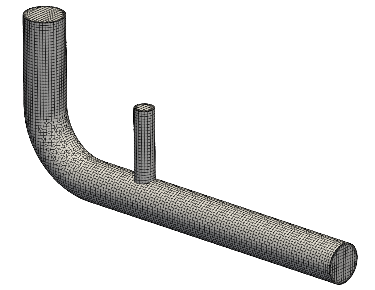
At this point the mesh generation is complete. The mesh consists of:
- Background mesh with a cell size of \(3 \text{mm}\)
- Five inflation layers at the walls with a thickness ratio of 1.3.
- Correct patch types for air and exhaust inlet, outlet, and pipe walls.
Mesh Quality
Once the mesh has been created, it is always recommended to check the mesh statistics and quality. This can easily be done using the utility checkMesh from within the exhaust_gas_recirculation folder:
checkMesh
The most relevant output is as follows:
// * * * * * * * * * * * * * * * * * * * * * * * * * * * * * * * * * * * * * //
Create time

Create polyMesh for time = 0

Time = 0s

Mesh stats
    points:           66681
    faces:            190868
    internal faces:   181436
    cells:            62182
    faces per cell:   5.98733
    boundary patches: 5

...

Checking geometry...
    Overall domain bounding box (-20.0004 -170 -19.9912) (360 7.23793e-11 19.9912)
    Mesh has 3 geometric (non-empty/wedge) directions (1 1 1)
    Mesh has 3 solution (non-empty) directions (1 1 1)
    Boundary openness (4.74107e-17 -7.05875e-17 -2.54233e-15) OK.
    Max cell openness = 5.20632e-16 OK.
    Max aspect ratio = 16.3738 OK.
    Minimum face area = 0.206012. Maximum face area = 13.7709.  Face area magnitudes OK.
    Min volume = 0.177828. Max volume = 37.082.  Total volume = 627526.  Cell volumes OK.
    Mesh non-orthogonality Max: 61.6751 average: 6.22186
    Non-orthogonality check OK.
    Face pyramids OK.
    Max skewness = 2.4353 OK.
    Coupled point location match (average 0) OK.


Mesh OK.

End
This gives us all relevant mesh statistics and quality criteria of the mesh:
- The mesh consists of 62182 cells,
- has 5 different boundary patches,
- the overall boundingbox of \(380\,\text{m}\) in \(x\)-direction, \(170\,\text{m}\) in \(y\)-direction and \(40\,\text{m}\) in \(z\)-direction.
As this is a hexa-dominant, unstructured mesh with five layers of inflation cells on the wall surfaces, the mesh quality in general is good:
- max cell aspect ratio of 16.4,
- a maximum mesh non-orthogonality of 61.7, and
- a max cell skewness of 2.44.
The final output Mesh OK. indicates that no critical problems or errors were found during checkMesh. Therefore, we can continue with this mesh and proceed with the simulation.
Mesh Scaling
The overall bounding box of the computational mesh does not match the given dimensions of the geometry, since the latter was created in millimeters. Therefore, the mesh has to be scaled down in all three directions with a scaling factor of \(0.001\). In order to do so, the mesh manipulation utility transformPoints can be used as follows:
transformPoints -scale "(0.001 0.001 0.001)"
If this command is executed twice, the mesh will be scaled by \(0.001 \times 0.001 = 10^{-6}\)!
Physical Properties
Thermophysical models are concerned with:
- Thermodynamics, e.g. relating internal energy \(e\) to temperature \(T\)
- Transport, e.g. the dependence of properties such as viscosity \(\mu\) on temperature
- State, e.g. dependence of density on temperature \(T\) and pressure \(p\).
Unlike the setup for incompressible flows, these thermophysical properties are stored in the thermophysicalProperties file in the constant directory.
A thermophysical model required an entry named thermoType which specifies the package of thermophysical modelling that is used in the simulation. OpenFOAM includes a large set of pre-compiled combinations of modelling, built within the code using C++ templates.
The individual submodels chosen for this case are as follows:
// * * * * * * * * * * * * * * * * * * * * * * * * * * * * * * * * * * * * * //

thermoType
{
    type            hePsiThermo;
    mixture         pureMixture;
    transport       const;
    thermo          hConst;
    equationOfState perfectGas;
    specie          specie;
    energy          sensibleEnthalpy;
}
Depending on these submodels, specific fluid properties have to be specified. These settings are within the mixture dictionary in the thermophysicalProperties file:
mixture
{
    specie
    {
        molWeight   28.9;
    }
    thermodynamics
    {
        Cp          1007;
        Hf          0;
    }
    transport
    {
        mu          1.8e-5;
        Pr          0.7;
    }
}
Composition of each constituent
There is currently only one option for the specie model which specifies the composition of each constituent. That model is itself named specie, which is specified by the entry molWeight, which specifies the grams per mole of the given species. Here, air is considered with a mol weight of \(28.9\,\text{g/mol}\).
Thermodynamics model
The thermodynamic models are concerned with evaluating the specific heat \(c_p\) from which other properties are derived. The thermodynamics model selected here is of type hConst, which assumes a constant \(c_p\) and heat of fusion \(H_f\), which is simply specified by two keywords, cp set to \(1007\,\text{J/(kg K)}\) and Hf set to \(0\).
Equation of state
The equation of state for the given fluid is set to perfect gas. Therefore, density is calculated based on the following relation without the need of any additional material parameter:
\[\rho = \frac{p}{R\,T}\]with the specific gas constant for air \(R\).
Transport model
The transport modelling concerns evaluating dynamic viscosity \(\mu\), thermal conductivity \(\kappa\), and thermal diffusivity \(\alpha\). In this case, a const transport model is specified, which assumes a constant dynamic viscosity \(\mu\) and Prandtl number \(\text{Pr}\). These two variables are specified by the keywords mu set to \(1.8 \times 10^{-5}\) and Pr to \(0.7\). Since thermal conductivity and thermal diffusivity can be derived from these quantities, they do not have to be specified.
Turbulence Modelling
The turbulence model is set in the turbulenceProperties file in the constant directory. The content of the file is as follows:
simulationType RAS;

RAS
{
    RASModel        kOmegaSST;
}
For this set of simulation the Reynolds-Averaged Navier-Stokes (RANS) equations should be solved. Therefore, the entry simulationType is set to RAS, which stands for Reynolds-Averaged Simulation. Within the RAS sub-dictionary, the keyword RASModel set to kOmegaSST selects the SST \(k-\omega\) turbulence model.
Boundary Conditions
Since the simulation starts at time \(t=0\), the boundary and initial field data is stored in the 0 sub-directory. This must be done for all variables solved for, such as pressure p, velocity U and temperature T as this is a compressible case. Furthermore, the SST \(k-\omega\) solves two additional transport equations for turbulent kinetic energy \(k\) and specific dissipation rate \(\omega\). Therefore, initial and boundary conditions have to be provided for these variables as well. Finally, the treatment of the turbulent viscosity \(\nu_\text{t}\) and turbulent thermal diffusivity \(\alpha_\text{t}\) at the walls have to be specified as well.
Pressure, Velocity and Temperature
For this example case, the volumetric flow rate at the air inlet as well as exhaust gas inlet are given. Instead of manually calculating the inlet velocity based on patch area (e.g., inlet velocity equal to volumetric flow rate divided by patch area), we can use the velocity inlet boundary condition flowRateInletVelocity and directly specify the volumetric flow rate. The setup for both inlets looks as follows:
inlet_air
{
    type                flowRateInletVelocity;
    volumetricFlowRate  0.005;
    value               uniform (0 0 0);
}

inlet_exhaust
{
    type                flowRateInletVelocity;
    volumetricFlowRate  0.0025;
    value               uniform (0 0 0);
}
Pressure at the inlet is treated as zero gradient and inlet temperature is \(300\,\text{K}\) for the air inlet and \(900\,\text{K}\) for the exhaust gas inlet, respectively. At the outlet, velocity and temperature are treated as zero gradient and the static pressure is set to \(10^5\,\text{Pa}\). The walls are considered no-slip and adiabatic. Thus, the velocity is set to \((0 \, 0 \, 0)\), temperature and pressure to zero gradient.
Turbulent Quantities
The turbulent kinetic energy \(k\) at the inlet is estimated based on turbulent intensity \(I_t\) using the turbulentIntensityKineticEnergyInlet boundary condition with an intensity of 2 % at the air inlet and 8 % at the exhaust gas inlet. Similarly, specific dissipation rate \(\omega\) is estimated via turbulent length scale \(L_t\) and the turbulentMixingLengthFrequencyInlet boundary condition. In both cases, the length scale is equal to the pipe diameter. Wall functions are used for the walls with the kqRWallFunction for turbulent kinetic energy and the omegaWallFunction for the specific dissipation rate. At the outlet, both variables are treated with zero gradient. Turbulent kinetic energy and specific dissipation rate are initialized with \(0.1\,\text{m}^2\text{/s}^2\) and \(10\,000\,\text{1/s}\), respectively.
Turbulent viscosity \(\nu_t\) and turbulent thermal diffusivity \(\alpha_t\) have to be specified only at the walls. Here, we are using a wall funtion approach as well with the nutUSpaldingWallFunction boundary condition for mut and the compressible::alphatWallFunction boundary condition for alphat. All other patches are set to calculated as they will be computed by the turbulence model itself.
Simulation Control
Settings related to the control of time and reading and writing of the solution data are read in from the controlDict file in the system folder.
The key settings for this steady-state turbulent simulation include:
application     rhoPimpleFoam;

startTime       0;

stopAt          endTime;

endTime         0.08;

deltaT          8e-6;

writeControl    runTime;

writeInterval   0.002;
In this tutorial case, the solver rhoPimpleFoam is used, a pressure-based solver for compressible, transient, laminar or turbulent single-phase flows. The simulation starts at time 0. Therefore we set the startFrom keyword to startTime and then specify the startTime keyword to be 0. The simulations runs until an end time of \(0.08\,\text{s}\). Time step size deltaT is set to \(8 \times 10^{-6}\,\text{s}\) for stability reasons. Finally, results are witten out every \(0.002\,\text{s}\) configured via the writeInterval keyword.
Discretization
The user specifies the choice of finite volume discretisation schemes in the fvSchemes dictionary in the system directory. Here, we will only cover the most relevant settings.
Temporal derivatives
The discretization of the temporal derivatives \((\partial / \partial t)\) is defined within the ddtSchemes keyword. The entry here is set to Euler, e.g. a first order implicit time discretization.
ddtSchemes
{
    default             Euler;
}
Gradient terms
The discretization of the gradient terms is defined within the gradSchemes keyword. All gradient schemes are discretized equally with a second order central differencing scheme. Hence, the default discretization is set to Gauss linear.
gradSchemes
{
    default             Gauss linear;
}
Convective terms
The discretization of the convective transport terms is defined within the divSchemes keyword. The convective transport of momentum div(phi,U) adn enthalpy div(phi,h) is discretized using the second order upwind scheme called Gauss linearUpwind combined with the default gradient scheme defined under gradSchemes. The convection of kinetic energy in the energy equation div(phi,K) is discretized with a second order central differencing scheme called Gauss linear and the turbulent quantities are discretized with first order upwind.
Additionaly, div((nuEff*dev2(T(grad(U))))) denotes the divergence of the shear stress tensor in the momentum equation. Since this term is diffusive in nature, it is recommended to discretize it with a central differencing scheme, here Gauss linear.
divSchemes
{
    div(phi,U)      Gauss linearUpwindV default;

    div(phi,h)      Gauss linearUpwind default;
    div(phi,K)      Gauss linear;

    div(phi,k)      Gauss upwind;
    div(phi,omega)  Gauss upwind;

    div(((rho*nuEff)*dev2(T(grad(U))))) Gauss linear;
}
Linear Solver Settings
The specification of the linear equation solvers, tolerances and other algorithm controls is made in the fvSolution dictionary in the system directory. These settings are as follows for the exhaust gas recirculation case.
Solver settings
The pressure field in the pressure-velocity coupling is solved using a Geometric agglomerated Algebraic MultiGrid (short: GAMG) solver with a Gauss-Seidel solver for smoothing during the multi-grid steps. The solver is actually set up twice as the pressure-velocity equation is solved more than once. For the intermediate iterations, a relative tolerance of \(0.01\) is used while for the final iteration a relative tolerance of \(0\) is used.
solvers
{
    p
    {
        solver          GAMG;
        smoother        GaussSeidel;
        tolerance       1e-06;
        relTol          0.01;
    }

    pFinal
    {
        $p;
        relTol          0;
    }
...
}
The momentum and energy equation as well as the transport equations for the turbulent properties are solved using a Gauss Seidel solver . The absolute tolerance for solving is \(10^{-6}\) with a relative tolerance of \(0.1\):
solvers
{
...

    "(rho|U|h|k|omega)"
    {
        solver          smoothSolver;
        smoother        symGaussSeidel;
        tolerance       1e-06;
        relTol          0.1;
    }

    "(rho|U|h|k|omega)Final"
    {
        $U;
        relTol          0;
    }
}
Pressure-velocity coupling
Pressure-based, steady-state simulations in OpenFOAM rely on the PIMPLE pressure-velocity coupling algorithm. Additional options for this algorithm are available within the PIMPLE entry in fvSolutions. In this tutorial, the pressure correction equation is solved one additional time every iteration for improved convergence and stability with the nCorrectors entry set to 2. Since this is a transient simulation, relaxation factors or residual criteria are not necessarily required.
PIMPLE
{
    nOuterCorrectors    1;
    nCorrectors         2;
    nNonOrthogonalCorrectors 0;
}