Solving

Starting the Solver

In order to start the simulation, we have to execute corresponding the OpenFOAM application. As defined in the controlDict, the solver pimpleFoam will be used, suitable for transient, incompressible, laminar or turbulent flows. This application can be started by typing the appropriate command in the terminal from within the case directory:

pimpleFoam

The progress of the job is written to the terminal window. It tells the user the current time step, the equations being solved, initial and final residuals for all fields and should look like follows:

Courant Number mean: 0.148717 max: 0.590908
Time = 0.081

PIMPLE: iteration 1
smoothSolver:  Solving for Ux, Initial residual = 0.000976598, Final residual = 1.01157e-07, No Iterations 2
smoothSolver:  Solving for Uy, Initial residual = 0.0020057, Final residual = 2.55499e-07, No Iterations 2
GAMG:  Solving for p, Initial residual = 0.004064, Final residual = 1.60952e-05, No Iterations 4
time step continuity errors : sum local = 1.04098e-09, global = 2.08309e-10, cumulative = 2.1952e-07
GAMG:  Solving for p, Initial residual = 0.000712041, Final residual = 4.6156e-08, No Iterations 8
time step continuity errors : sum local = 2.97078e-12, global = 4.48358e-13, cumulative = 2.19521e-07
ExecutionTime = 4.04 s  ClockTime = 4 s

This output at time step 0.081 seconds tells us in summary:

• The maximum Courant number of the simulation is 0.591 with an average value of 0.148. While being larger than the initially estimated (!) value of 0.25, it, is still smaller than 1.0 indicating a stable and accurate simulation.
• The smoothSolver (e.g., a Gauss-Seidel solver) is used to solve the velocity components Ux and Uy in \(x\)- and \(y\)-direction. In this time step, it takes 2 iterations to reach the specified residual criteria.
• The GAMG multigrid solver is used for solving the pressure poisson equation in the pressure-velocity coupling algorithm. For better stability and convergence, the pressure equation is solved twice per time step.
• The error of the conservation of mass is denoted as continuity error. Since its value is very small, conservation of mass is maintained.
• The execution time for the simulation up until this time step is 4.04 seconds as indicated by the ExecutionTime.

Monitoring the Simulation

In order to track and monitor the simulation during its run, a function object is added at the bottom of the controlDict. These are used for e.g. writing out the residuals over the course of the simulation, perform certain post-processing tasks such as calculating the flow rate over a patch, compute maximum and average values of the flow field, compute forces and force coefficients on objects, compute derived fields such as heat transfer or shear stress rates, and generate images through cutPlanes or iso-surfaces. In this case, the controlDict looks as follows:

functions
{
    solverInfo
    {
        type            solverInfo;
        libs            (utilityFunctionObjects);
        fields          (p U);
    }
}

Plotting the Residuals

By default, the residuals are only printed to the terminal window. In order to visualize the residuals to help judge convergence, a function object has been added to the controlDict. This function object of type solverInfo saves the initial residuals of the fields (p U), so pressure and velocity, during runtime. Therefore, a new folder called postProcessing is automatically created inside the case folder. So in this example, the residuals are stored under the following path: postProcessing/solverInfo/0/solverInfo.dat.

Once the simulation has finished and all the time directories are written out, the data written by the function objects can be analyzed. This data can typically be plotted in a diagram using Microsoft Excel, Python, Gnuplot or any other tool. In order to quickly evaluate the monitored results from the function objects, a script is added to the backward-step case directory called create_plots.py. Executing it will automatically create the diagrams for residuals and average inlet pressure after the run. By typing the following command in the terminal, the diagrams are created using Python and stored as png file:

python3 create_plots.py

This creates the following diagram of the residuals on the \(y\)-axis plotted against the simulation time on the \(x\)-axis in the case folder:

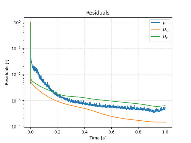
The plot shows that the residuals fall throughout the simulation to the range of \(10^{-4}\) for pressure and velocity. Running the simulation for longer would probably reduce the residuals even further.