Post-Processing

Visualizing the Results

As soon as results are written to time directories, they can be viewed using ParaView. Start ParaView in the background with the following command:

paraFoam &

To prepare ParaView to display the data of interest, the data at the required iteration of 547 must be loaded. If the case was run while ParaView was open, the output data in time directories will not be automatically loaded within ParaView. To load the data the user should click Refresh at the top Properties window (scroll up the panel if necessary).

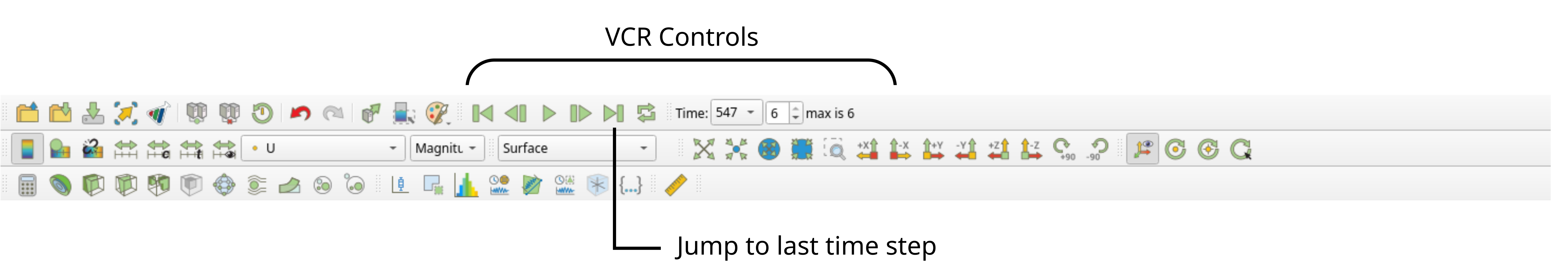
The solution at the iteration 547 can be viewed by using the VCR Controls at the very top of the ParaView window and click the button for Last Frame.

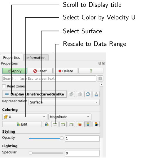
To color the mesh by velocity magnitude (i.e. the velocity contour) of the flow, the following settings must be selected in the Properties panel, as descriped in the following figure:

1. Select Surface from the Representation menu,
2. Select Coloring by velocity magnitude U at the cell centers, and
3. Select Rescale to Data Range, if necessary.

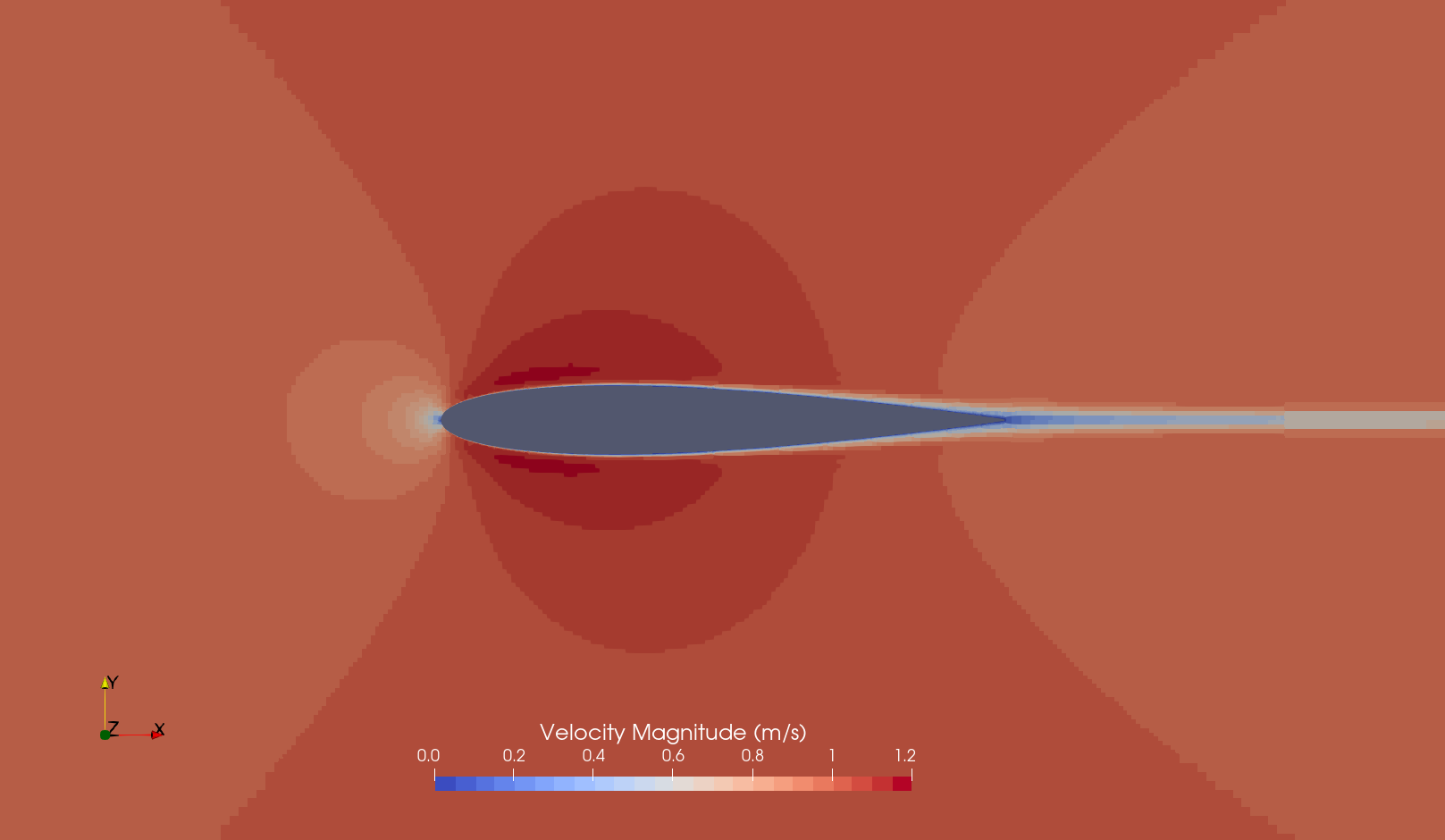
We can clearly see the flow around the airfoil the following key flow features: (1) Stagnation point at the airfoil leading edge, (2) fluid acceleration at the upper and lower surface (symmetric), (3) a thin, symmetric wake downstream, and (4) a symmetric pressure distribution about the chord line.

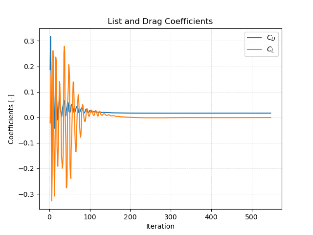
Force Coefficients

We have used the force coefficients to judge convergence. However, we can also use the values for validation. However, the force coefficients plot is not suited for that since we cannot get exact values from it:

Instead, we can open the file postProcessing/forceCoeffs/0/coefficient.dat and get the raw coefficients and compare it with experimental or analytical values. Compared to the XFoil airfoil database, the results look like follows:

Coefficient	Simulation	XFoil
Drag	0.0169	0.0169
Lift	-0.0007	0.0000

The results reveal a very good agreement for the NACA 0012 airfoil simulation at zero angle of attack.

Conclusion

This concludes the third seminar on the simulation of incompressible, laminar flow over around an airfoil. A two-dimensional mesh was generated using cartesian2DMesh based on a geometry file. The inlet boundary condition for velocity was adjusted to match a specified Reynolds number. The simulation was then run using simpleFoam, and residuals and force coefficients were plotted. Finally, the flow field was visualized in ParaView.