Post-Processing

Visualizing the Velocity Contour

As soon as results are written to time directories, they can be viewed using ParaView. Start ParaView in the background with the following command:

paraFoam &

To prepare ParaView to display the data of interest, the data at the required iteration of 547 must be loaded. If the case was run while ParaView was open, the output data in time directories will not be automatically loaded within ParaView. To load the data the user should click Refresh at the top Properties window (scroll up the panel if necessary).

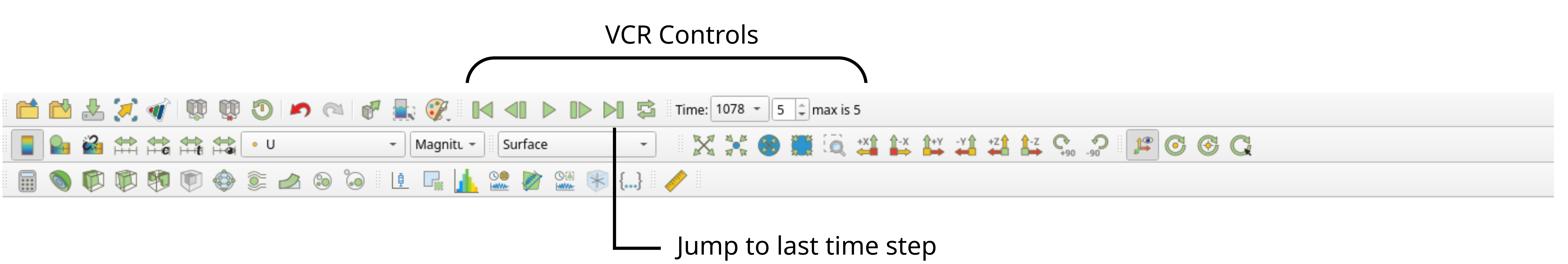
The solution at the iteration 1078 can be viewed by using the VCR Controls at the very top of the ParaView window and click the button for Last Frame.

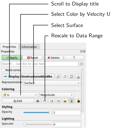
To color the mesh by velocity magnitude (i.e. the velocity contour) of the flow, the following settings must be selected in the Properties panel, as descriped in the following figure:

Select Surface from the Representation menu,
Select Coloring by velocity magnitude U at the cell centers, and
Select Rescale to Data Range, if necessary.

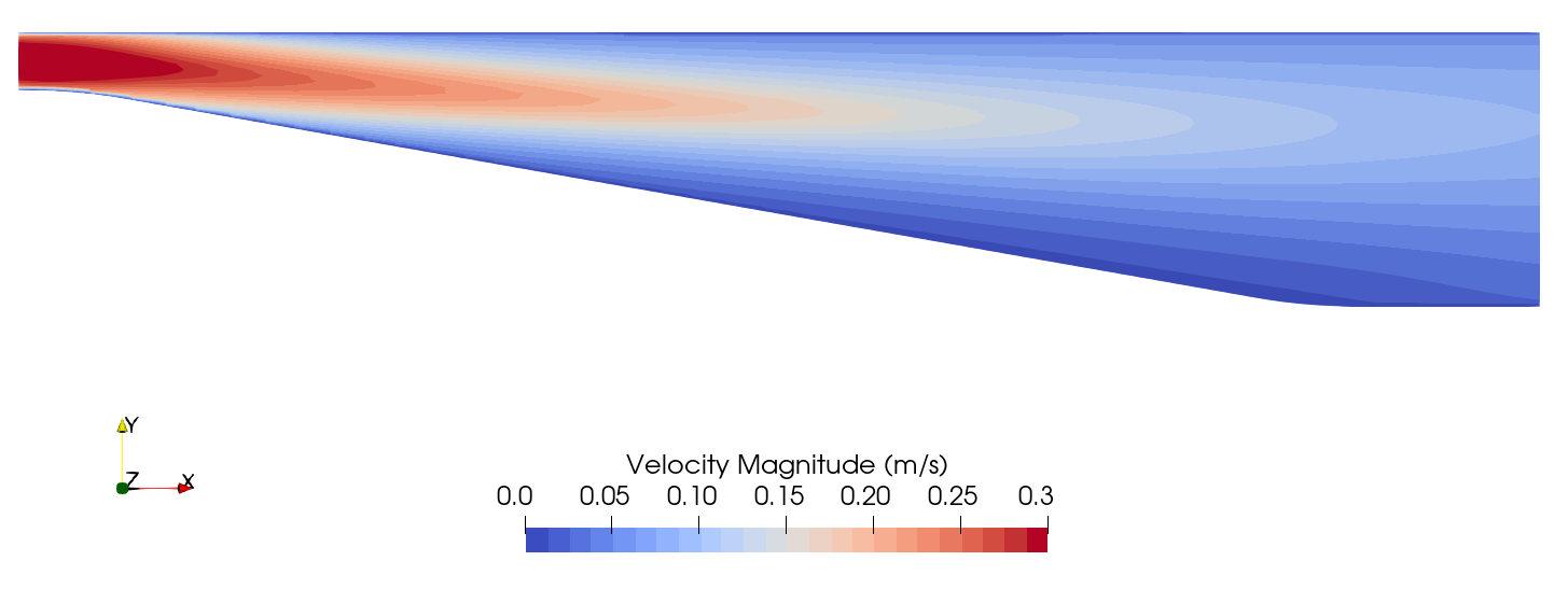
When inspecting the velocity field through the diffuser, the reduction in flow velocity due to the incresed cross-sectional area is apparent. Furthermore, no recirculation is noticable at the lower end of the diffuser, something which would be expected due to the large opening angle of the diffuser.ine.

Diffuser paraview velocity contour

Visualizing Flow Streamlines

Streamlines of the flow field are a great way of visualizing any possible recirculation. With the diffuser.foam module highlighted in the Pipeline Browser, select the Stream Tracer filter from the Common Data and Analytics menu. The Properties window panel should appear as shown in the following figure:

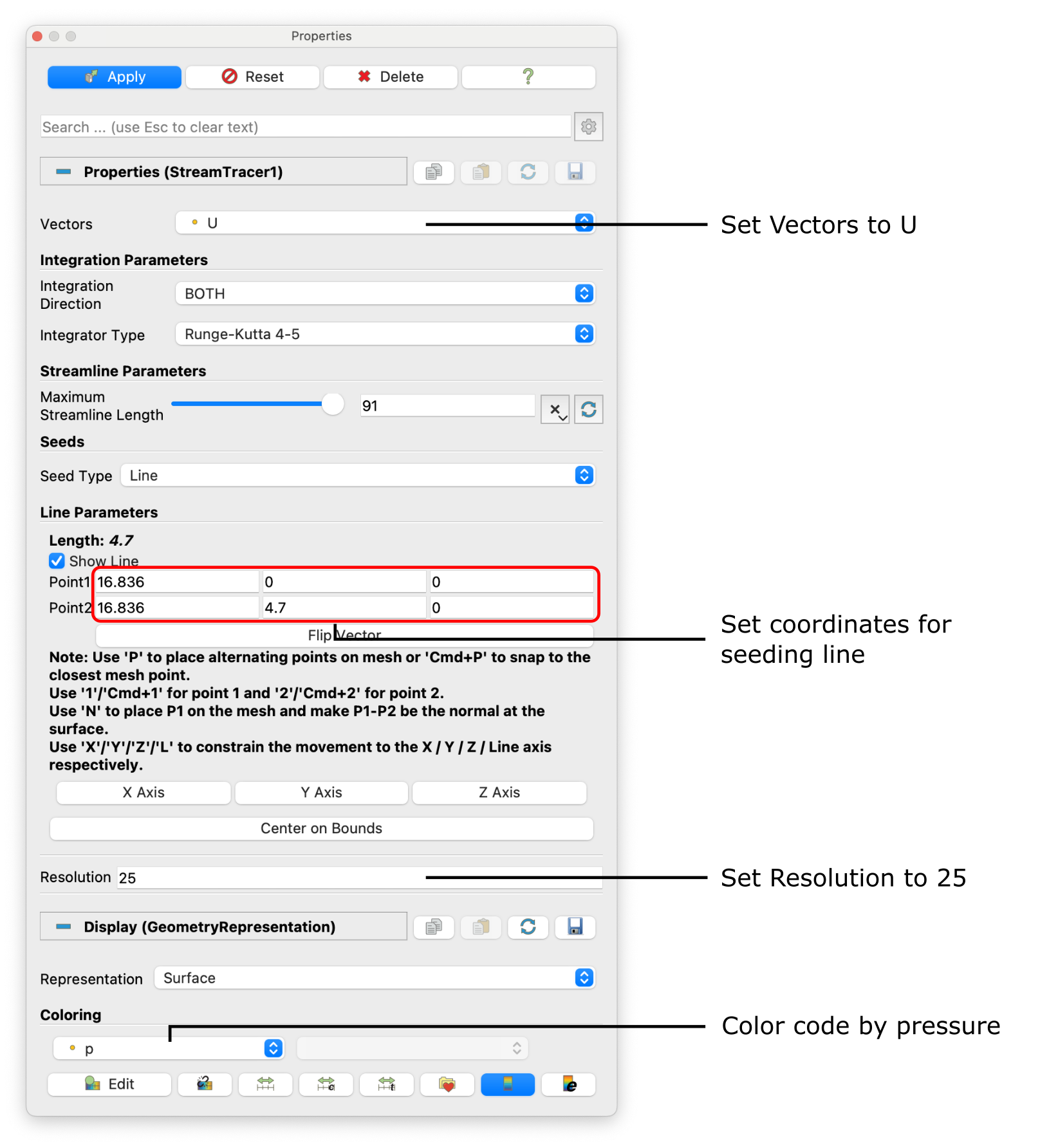
In the resulting Properties panel, make sure the stream lines are plotted according to the velocity vector field U. Streamlines are seeded along a straight line with the starting point \((16.836 \,\, 0\,\, 0)\) and end point \((16.836 \,\, 4.7\,\, 0)\) with a Seeding Resolution of 25 streamlines along this straight line. Finally, color code the streamlines by pressure p. Click Apply to show the streamlines through the diffuser as follows:

Diffuser paraview stream tracer

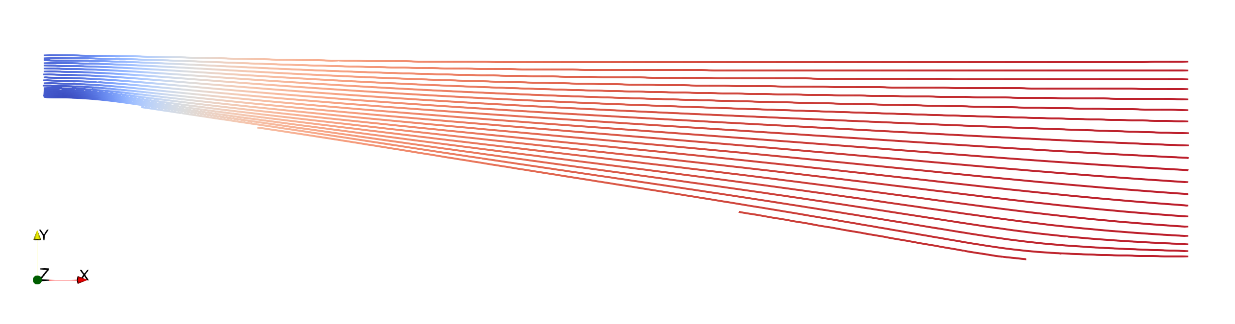
The adverse pressure gradient with an increase in pressure along the streamlines is clearly visible and there is no flow separation and recirculation at the lower wall. However, adverse pressure gradients and flow separation are the weakpoints of the standard \(k-\epsilon\) turbulence model.

Plotting the Velocity Profile

For a better comparison with experimental data, a vertical velocity profile of the \(x\)-velocity component is recommended. For this, hide the StreamTracer filter in the Pipeline Browser by clicking the eye icon next to it and only show the original case named diffuser.foam. Now, select the Plot over Line filter from the Domain \(\rightarrow\) Data Analysis. The Properties window panel should appear as shown in the following figure:

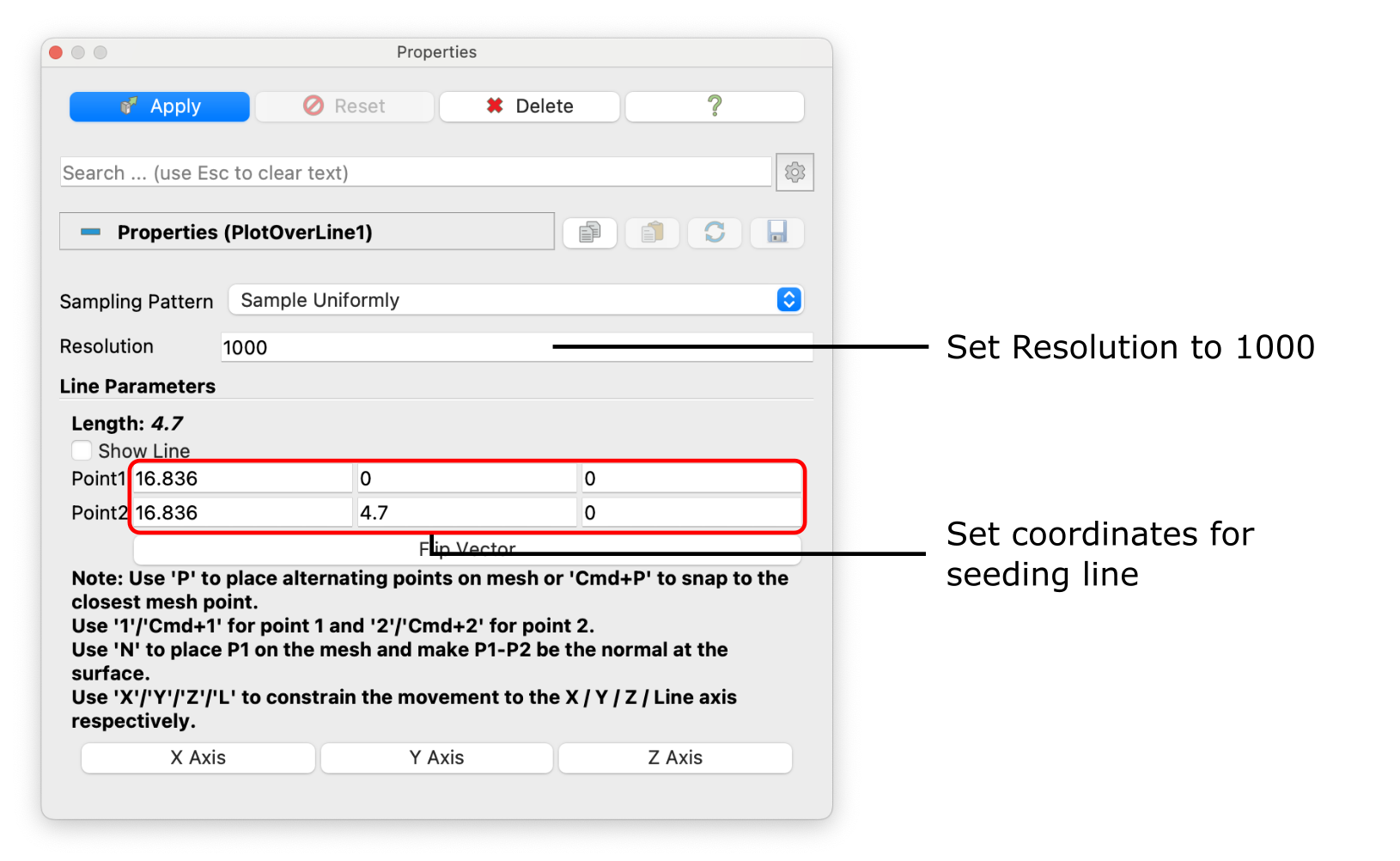
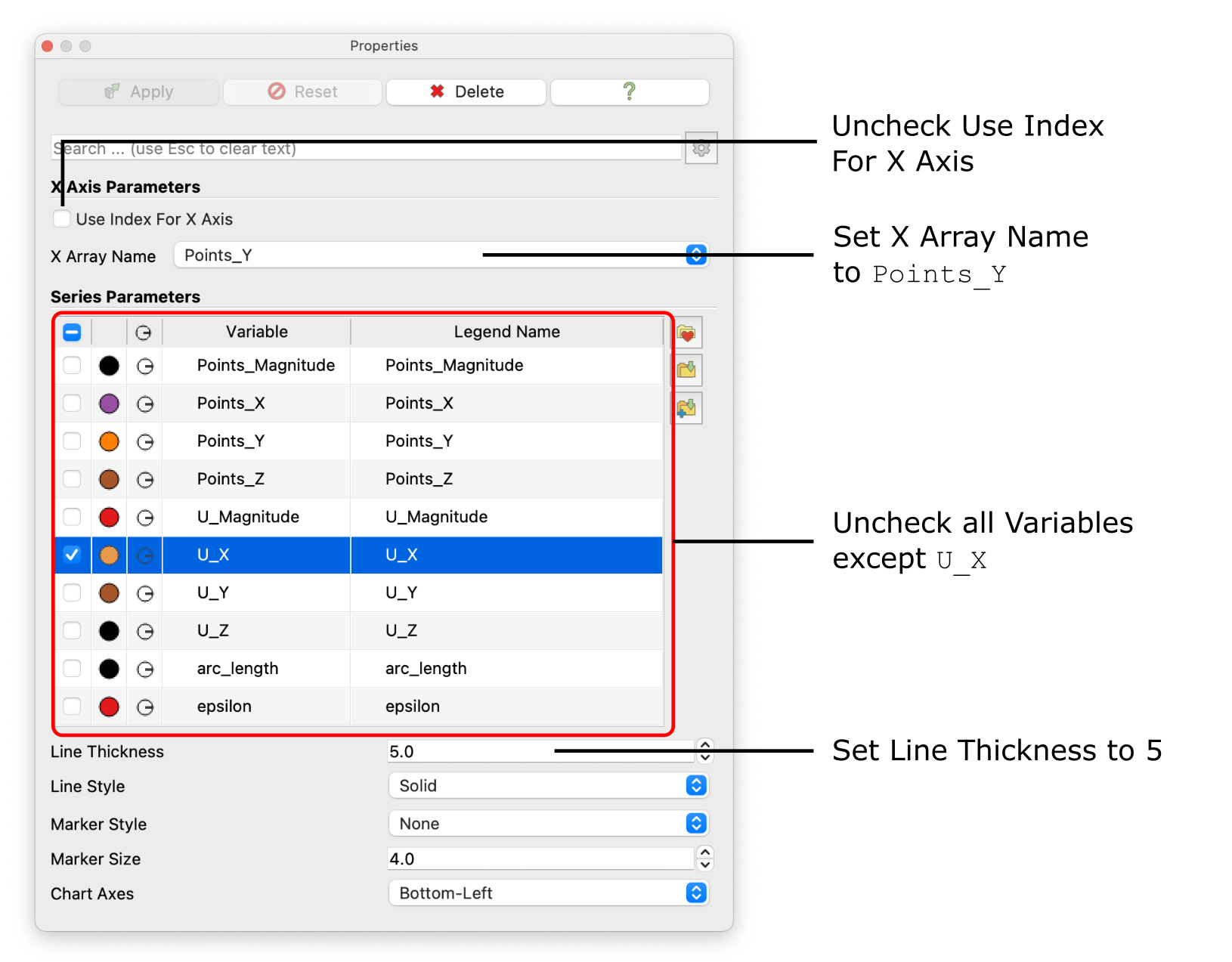
Similar to the streamlines, the coordinates of the start and end point of the sampling line should be \((16.836 \,\, 0\,\, 0)\) and \((16.836 \,\, 4.7\,\, 0)\), respectively, with a spatial Resolution of 1000 points along this line. Clicking Apply will open a separate window plotting all variables solved over the length of the line. This resulting diagram is very cluttered. Therefore, in the Properties window deselect all variables except the \(x\)-velocity component labelled U_X. In order to plot over the \(y\)-coordiantes of the line, uncheck Use Index for X Axis and set X Array Name to Points_Y. Finally, thile the \(x\)-velocity component is selected in the Properties window, change the Line Thickness to 5 for better readability. Optionally, line color can be changed and chart title as well as axis can be specified. The Properties window should now look like follows:

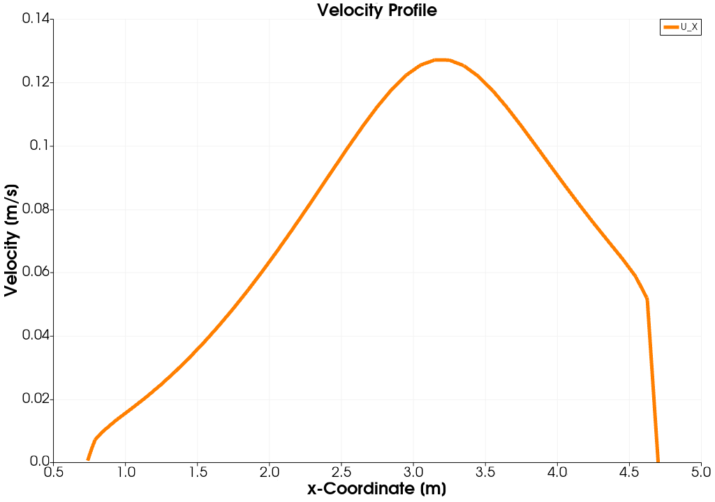
The resulting diagram should look like follows:

Validating the Results

Fortunately, experimental measurements are availabel in order to assess the accuracy of the numerical results. This data can be found in the file experiment.csv in the case folder. With the following steps, the experimental data will loaded into ParaView and plotted alongside the numerical velocity profile.

Click on Open… in the Files menu and select the file experiment.csv. Confirm the CSV Reader with OK and click Apply. A new Spreadsheet View should open showing the content of the file: Three columns of data with Row ID, velocity in meter per second, and \(y\)-coordinate.
Select on the previously created diagram in ParaView and click on the Eye icon next to the experiment.csv entry in the Pipeline Browser to show the content of the CSV-file in the diagram.
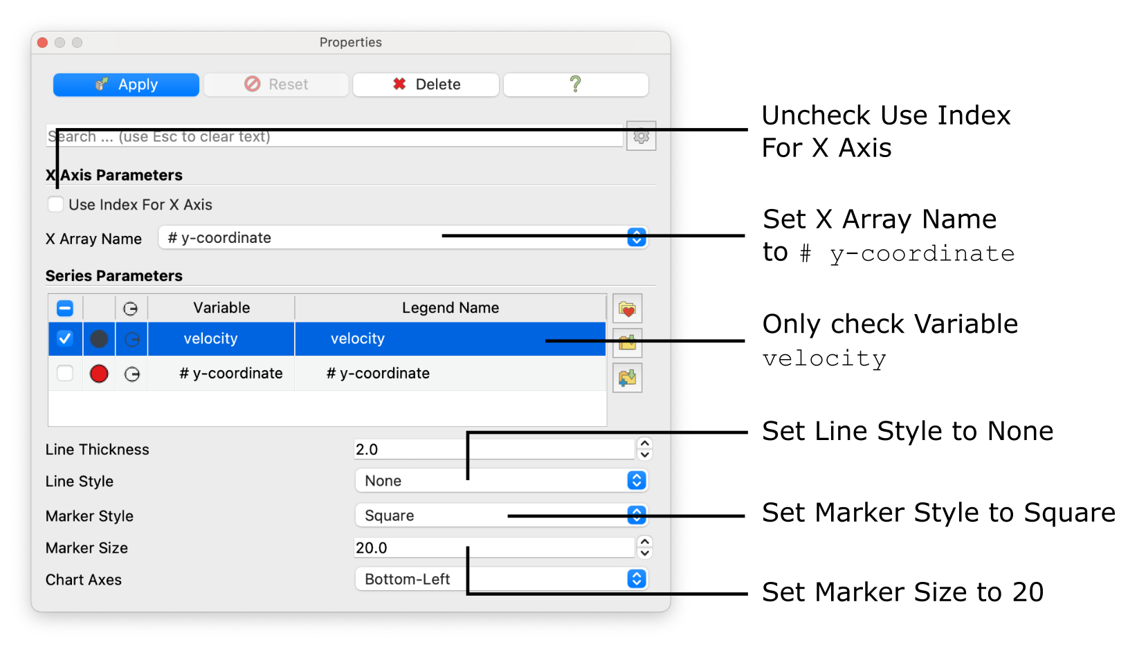
In order to plot velocity over \(y\)-coordiante, select the experiment.csv entry in the Pipeline Browser, set the X Array Name to # y-coordiante, only select the velocity in the Series Parameter list, set Line Style to None, Marker Style to Square, and Marker Size to 20. These settings are summarized in the following figure:

The resulting diagram should look like follows:

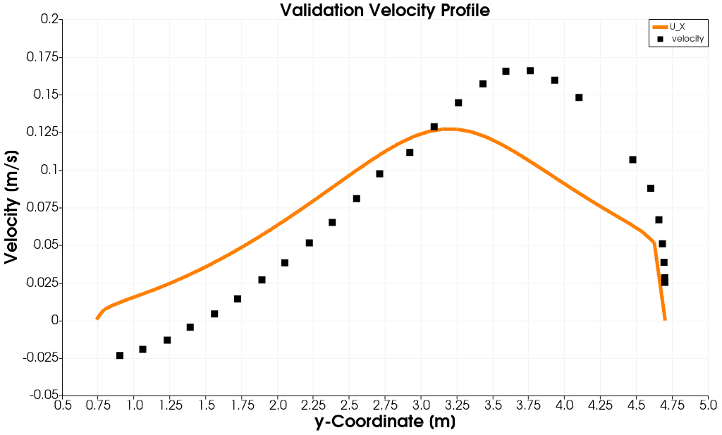
This results confirms the huge discrepancy between the experimentally measured velocity profile and the numerically simulated one. First, no flow separation and thus recirculation is predicted by the numerical model. Second, the maximum flow velocity in \(x\)-direction is significantly underpredicted. This confirms the previous statement that the standard \(k-\epsilon\) turbulence model is a poor choice for this flow problem.

Conclusion

This concludes the fourth seminar on the simulation of an incompressible, turbulent flow through a diffuser. A two-dimensional mesh was generated using cartesian2DMesh based on a geometry file. The boundary conditions were adjusted for the standard \(k-\epsilon\) turbulence model. The simulation was then run using simpleFoam, and residuals was plotted and dimensionless wall distance \(y^+\) evaluated. Finally, the flow field was visualized in ParaView and the velocity profile within the diffuser compared with experimental measurements revealing a huge modelling error due to the turbulence model.