Post-Processing

Visualizing the Velocity Contour

As soon as results are written to time directories, they can be viewed using ParaView. Start ParaView in the background with the following command:

paraFoam &

To prepare ParaView to display the data of interest, the data at the final time step of 1 second must be loaded. If the case was run while ParaView was open, the output data in time directories will not be automatically loaded within ParaView. To load the data the user should click Refresh at the top Properties window (scroll up the panel if necessary).

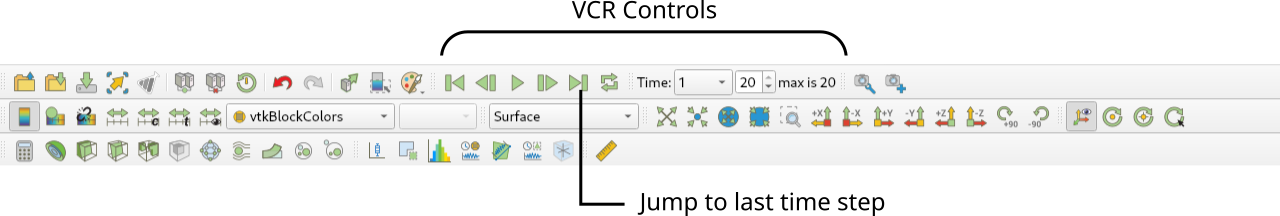
The solution at the last time step of \(t = 1\,\text{s}\) can be viewed by using the VCR Controls at the very top of the ParaView window and click the button for Last Frame

Coloring Surfaces by Flow Property

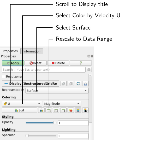
To color the mesh by velocity magnitude (i.e. the velocity contour) of the flow, the following settings must be selected in the Properties panel, as descriped in the following figure:

1. Select Surface from the Representation menu,
2. Select Coloring by velocity magnitude U at the cell centers, and
3. Select Rescale to Data Range, if necessary.

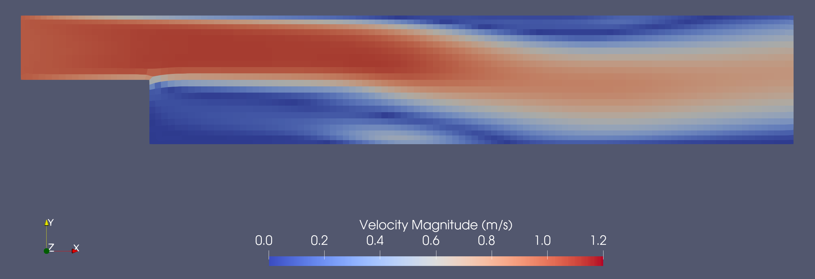
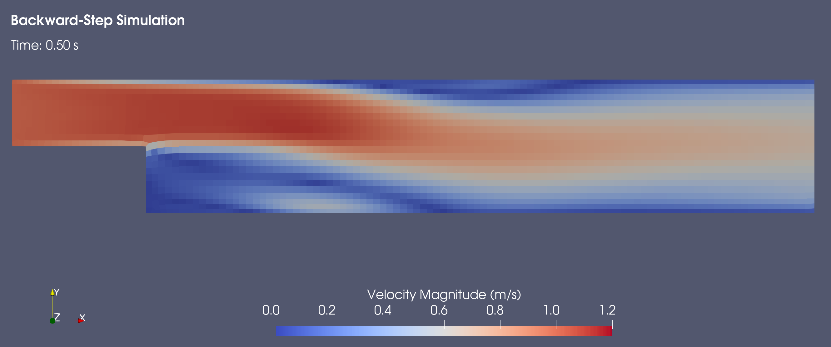
The velocity field looks as expected: The velocity magnitude at the inlet is about \(1\,\text{m/s}\). The flow separates at the step corner and there is a recirculation zone immediately downstream of the step. The flow rattaches to the bottom wall further downstream, after which a recovery region follows. The typical reattachment length is 6-8 step heights for a Reynolds number of 1250.

A colour legend can be added by clicking the Toggle Color Legend Visibility button in the Active Variable Controls toolbar. The legend can be located in the image window by drag and drop with the mouse.

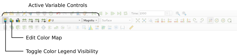
The Edit Color Map button in the Active Variable Controls toolbar opens the Color Map Editor window, where the user can set a range of attributes of the colour scale and the color bar.

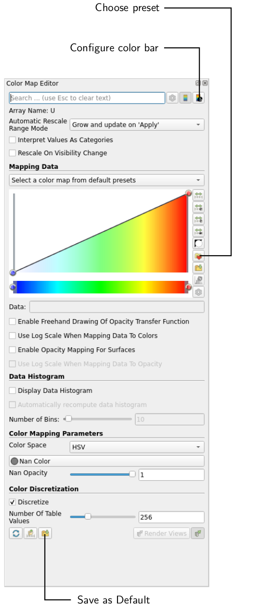
In particular, ParaView defaults to using a colour scale of blue to white to red rather than the more common blue to green to red (rainbow). Therefore the first time that the user executes ParaView, they may wish to change the colour scale. This can be done by selecting the Choose Preset button (with the heart icon) in the Color Map Editor. The conventional color scale for CFD is Blue to Red Rainbow can be found when the user types the name in the Search bar.

After selecting Blue to Red Rainbow and clicking Apply and Close, the user can click the Save as Default button at the absolute bottom of the panel (file save symbol) so that ParaView will always adopt this type of colour bar. The user can also edit the color legend properties, such as text size, font selection and numbering format for the scale, by clicking the Edit Color Legend Properties to the far right of the search bar, as shown in the figure above.

Cutting Plane (Slice)

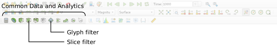
If the user rotates the image, by holding down the left mouse button in the image window and moving the cursor, they can see that they have now coloured the complete geometry surface by the velocity. In order to produce a genuine 2-dimensional contour plot the user should first create a cutting plane, or slice. With the backward-step.foam module highlighted in the Pipeline Browser, the user should select the Slice filter from Common Data and Analytics in the top menu of ParaView:

The cutting plane should be centred at \((0, 0, 0)\) and its normal should be set to \((0, 0, 1)\) (click the Z Normal button). By default, the pressure field will now be shown. The Show Plane in the Properties panel should be disabled as otherwise rotating the image with the mouse might change the plane orientation.

Vector Plot (Glyph)

We now wish to generate a vector glyph for velocity at the cutting plane. With the slice1 module highlighted in the Pipeline Browser, the user should select the Glyph filter from the Common Data and Analytics menu. The Properties window panel should appear as shown in the following figure:

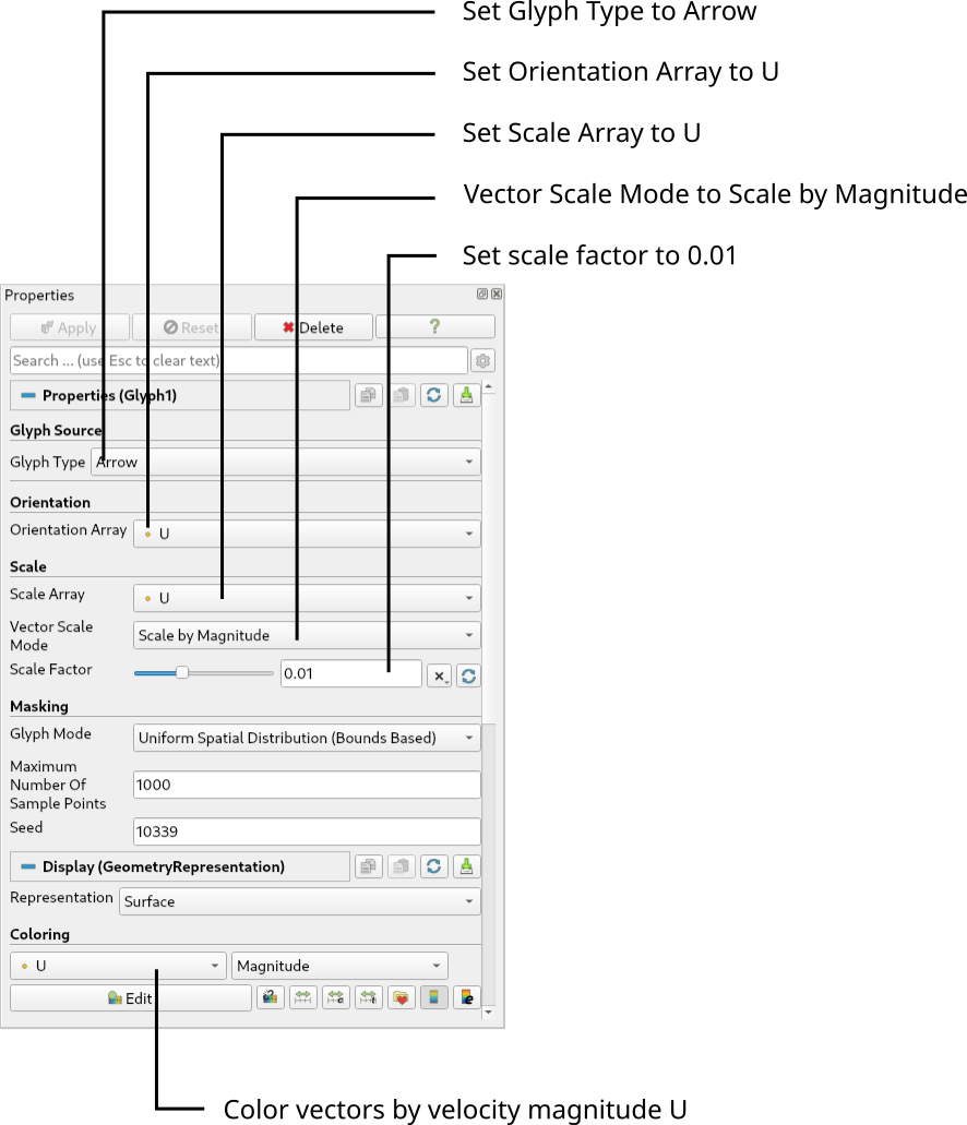
In the resulting Properties panel, make sure the Glyph Type is set to Arrow, and the Orientation Array is the velocity field U. Then, set the Scale Array to U and Vector Scale Mode to Scale by Magnitude. This way, the size of the vectors will be scaled by the velocity magnitude and with a Scaling Factor of 0.01 and the vectors will be clearly visible. At this point you can click Apply to show the vector plot on top of the Cutting plane defined previously.

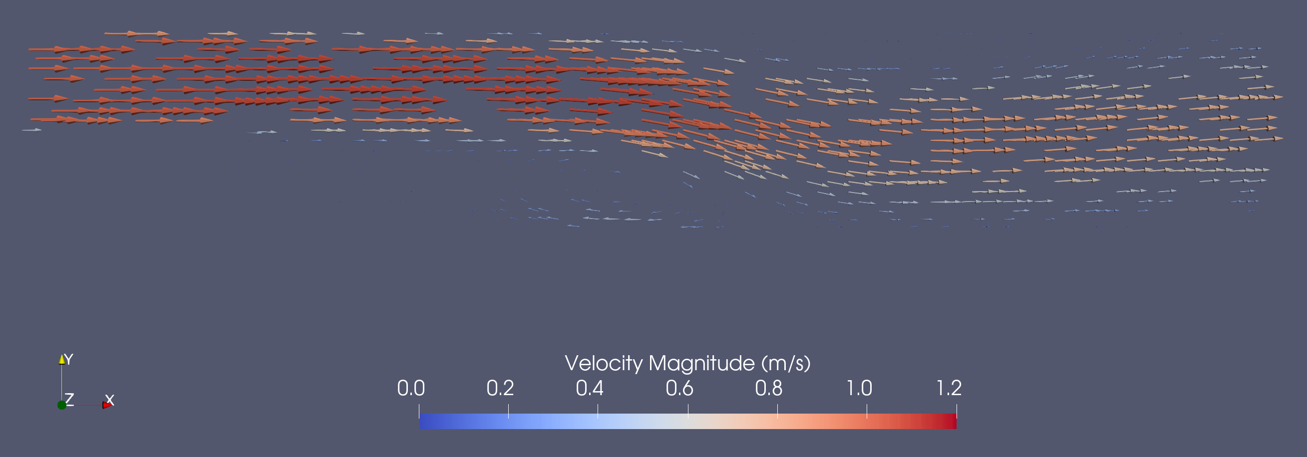
The resulting vectors will be color coded by pressure, whereas a velocity color code would make much more sense. Therefore, the user should colour the glyphs by velocity magnitude which, as usual, is controlled by setting Color by U in the Properties panel. The user can also select Show Color Legend in Edit Color Map. Additionally, the slice1 module in the Pipeline Browser can be made invisible by clicking the Eye symbol next to the module name. The resulting output is shown in the following figure:

Velocity Animation

A good way to visualize the transient flow behaviour is an animation created with ParaView. For this, hide the vector plot and show the cut plane of the velocity magnitude. Then display the velocity magnitude in a range from \((0 - 1.2) \, \text{m/s}\). By clicking the Play button at the VCR Controls at the very top, it is possible to automatically go through every time step and see what the transient flow field looks like:

Before creating an animation, it is recommended to add more information to the view. First of all, a title could be added by clicking on the top menu: Sources \(\rightarrow\) Annotations \(\rightarrow\) Text. You can type any text in the text field inside the Properties panel, adjust font size and location of the text field. Secondly, you could add the current time step to the view, again by using the top menu: Sources \(\rightarrow\) Annotations \(\rightarrow\) Annotate Time. Choose a suitable time Format, such as Time: {time:1.2f} s to display the time with two digits and the unit in seconds. All in all, this could look like follows:

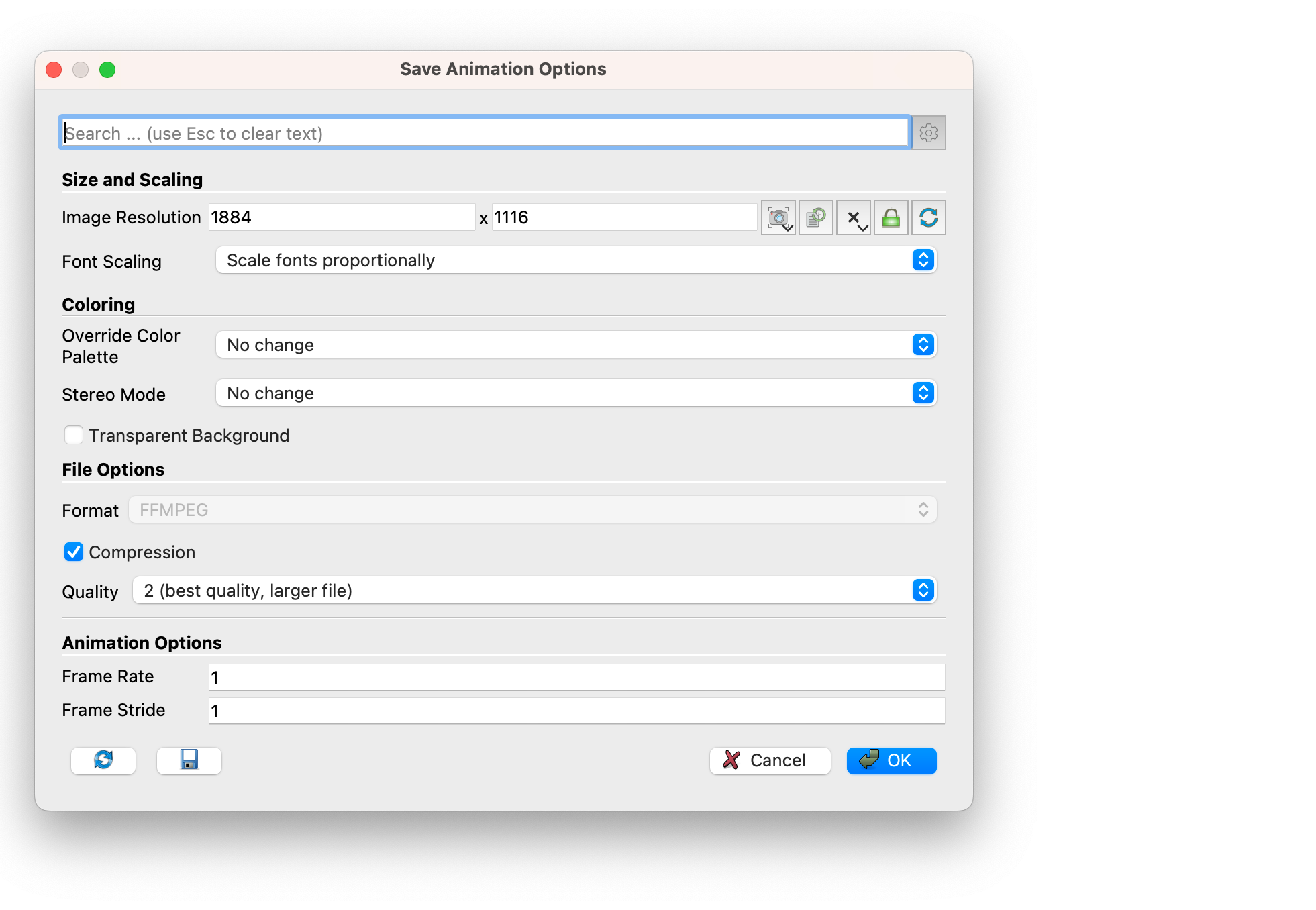
At this point, the animation can easily be created by clicking the top menu: File \(\rightarrow\) Save Animation…, and choosing a suitable file name and format (preferably mp4 or avi). At the following Animation Menu, you can specify video resolution, compression, and frame rate. It is recommended to change the frame rate to a higher value, such as 10 - 15. Clicking Okay will create the animation for you.

Conclusion

This concludes the second seminar on the simulation of incompressible, laminar flow over a backward-facing step. A two-dimensional mesh was generated using cartesian2DMesh based on a geometry file. The fluid properties were adjusted to match a specified Reynolds number, and the time step size was chosen to maintain an appropriate Courant number. The simulation was then run using pimpleFoam, and the residuals were plotted. Finally, the flow field was visualized in ParaView.