Pre-Processing
OpenFOAM Case Structure
A case being simulated involves data for mesh, fields, properties, control parameters, etc. In OpenFOAM this data is stored in a set of files within a case directory rather than in a single case file, as in many other CFD packages. The case directory is given a suitably descriptive name, here diffuser. This folder contains the following subfolders and files:
├── 0
│   ├── epsilon
│   ├── k
│   ├── nut
│   ├── p
│   └── U
├── constant
│   ├── turbulenceProperties
│   └── transportProperties
├── system
│   ├── controlDict
│   ├── fvSchemes
│   ├── fvSolution
│   └── meshDict
└── diffuser.stl

3 directories, 11 files
The relevant files for this tutorial case are:
0- This directory stores the initial values and boundary condition for each variables solved.constant- This directory contains files that are related to the physics of the problem, including the mesh and any physical properties that are required for the solver. In this case:turbulencePropertiesdefines, which turbulence model to use for the simulation
system- This folder contains files related to how the simulation is to be solved:controlDictfor setting control parameters including start/end time, time step size and parameters for data output.fvSchemesfor the discretization schemes used in the Finite Volume Method.fvSolutionfor the solver settings used in the Finite Volume Method.meshDictcontains the configuration for the automated meshing process.
Mesh Generation
The hexahedral-dominant, two-dimensional mesh is created automatically with the meshing utility cartesian2DMesh from a user provided surface geometry named `diffuser.stl, which is located in the case folder.
The diffuser has an initial channel height of \(H = 1\,\text{m}\) at the inlet and extends to \(4.7\,\text{m}\) towards the outlet. In order to achieve 10 cells across the channel height (exluding inflation layers), the maximum cell size is set to \(0.1\,\text{m}\). Additionally, the walls have a single inflation layer with a thickness ratio of 1.2. This way standard wall functions can be used by ensuring a dimensionless wall distance of \(y^+ > 30\).
The resulting meshDict looks as follows:
// * * * * * * * * * * * * * * * * * * * * * * * * * * * * * * * * * * * * * //

surfaceFile     "diffuser.stl";

maxCellSize     0.1;

boundaryLayers
{
    patchBoundaryLayers
    {
        "(lowerWall|upperWall)"
        {
            nLayers             1;

            thicknessRatio      1.2;
        }
    }
}
Finally, all corresponding patches are grouped together correctly using a suitable patch type. In order to create the mesh, the cartesian2DMesh utility has to be executed:
cartesian2DMesh
The resulting mesh can be visualized with ParaView should look like follows around the diffuser:
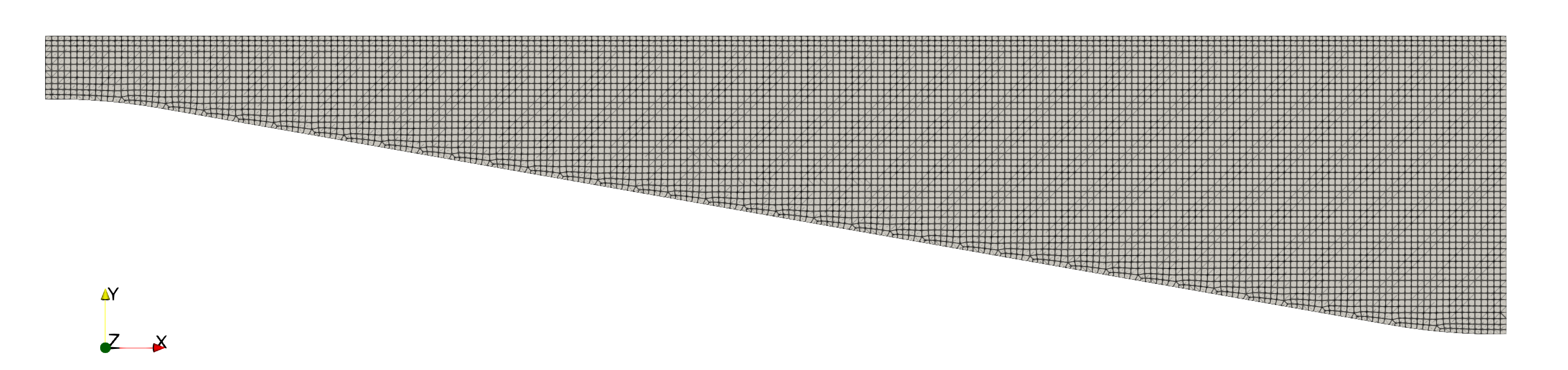
At this point the mesh generation is complete. The mesh consists of:
- Background mesh with a cell size of \(0.1 \text{m}\)
- A single inflation layer at the walls with a thickness ratio of 1.2.
- Correct patch types for inlet, outlet, lower and upper walls and front and back planes.
OpenFOAM always operates in a 3 dimensional Cartesian coordinate system and all geometries are generated in 3 dimensions. OpenFOAM solves the case in 3 dimensions by default but can be instructed to solve in 2 dimensions by specifying a special
emptyboundary condition on boundaries normal to the 3rd dimension for which no solution is required. Since the created mesh is two-dimensional, it will have a single cell layer in \(z\)-direction with the patchfrontAndBackPlanesof typeempty.
Mesh Quality
Once the mesh has been created, it is always recommended to check the mesh statistics and quality. This can easily be done using the utility checkMesh from within the diffuser folder:
checkMesh
The most relevant output is as follows:
// * * * * * * * * * * * * * * * * * * * * * * * * * * * * * * * * * * * * * //
Create time

Create polyMesh for time = 0

Time = 0s

Mesh stats
    points:           59346
    internal points:  0
    faces:            115814
    internal faces:   56470
    cells:            28714
    faces per cell:   6
    boundary patches: 5
    point zones:      0
    face zones:       0
    cell zones:       0

...

Checking geometry...
    Overall domain bounding box (-30 0 -0.651697) (61 4.7 0.651697)
    Mesh has 2 geometric (non-empty/wedge) directions (1 1 0)
    Mesh has 2 solution (non-empty) directions (1 1 0)
    All edges aligned with or perpendicular to non-empty directions.
    Boundary openness (-2.77203e-18 -1.50709e-16 9.20305e-15) OK.
    Max cell openness = 2.61181e-16 OK.
    Max aspect ratio = 1.58715 OK.
    Minimum face area = 0.00397046. Maximum face area = 0.155254.  Face area magnitudes OK.
    Min volume = 0.00517507. Max volume = 0.0143652.  Total volume = 362.148.  Cell volumes OK.
    Mesh non-orthogonality Max: 14.4587 average: 0.802326
    Non-orthogonality check OK.
    Face pyramids OK.
    Max skewness = 0.426205 OK.
    Coupled point location match (average 0) OK.

Mesh OK.

End
This gives us all relevant mesh statistics and quality criteria of the mesh:
- The mesh consists of 28714 cells,
- has 5 different boundary patches.
As this is a hexa-dominant, unstructured mesh with a single layer of inflation cells on the wall surfaces, the mesh quality in general is very good:
- max cell aspect ratio of 1.59,
- a maximum mesh non-orthogonality of 14.5, and
- a max cell skewness of 0.43.
The final output Mesh OK. indicates that no critical problems or errors were found during checkMesh. Therefore, we can continue with this mesh and proceed with the simulation.
Physical Properties
The physical properties for the fluid, such as kinematic viscosity, are stored in the transportProperties file in the constant directory.
Since the fluid is air, the kinematic viscosity is \(15 \times 10^{-6}\,\text{m}^2\text{/s}\) and set accordingly in the transportProperties dictionary as follows:
viscosityModel  Newtonian;

nu              15e-6;
Turbulence Modelling
The turbulence model is set in the turbulenceProperties file in the constant directory. The content of the file is as follows:
simulationType RAS;

RAS
{
    RASModel        kEpsilon;
}
For this set of simulation the Reynolds-Averaged Navier-Stokes (RANS) equations should be solved. Therefore, the entry simulationType is set to RAS, which stands for Reynolds-Averaged Simulation. Within the RAS sub-dictionary, the keyword RASModel set to kEpsilon selects the standard \(k-\epsilon\) turbulence model.
Boundary Conditions
Since the simulation starts at time \(t=0\), the boundary and initial field data is stored in the 0 sub-directory. This must be done for all variables solved for, such as pressure p and velocity U. Furthermore, the \(k-\epsilon\) solves two additional transport equations for turbulent kinetic energy \(k\) and turbulent dissipation rate \(\epsilon\). Therefore, initial and boundary conditions have to be provided for these variables as well. Finally, the treatment of the turbulent viscosity \(\nu_\text{t}\) at the walls has to be specified as well.
Pressure and Velocity
Since the Reynolds-number is set to \(\text{Re} = 2 \times 10^4\), a pressure-velocity boundary setup will be employed, where velocity is defined at the inlet while pressure is set at the outlet.
The velocity at the inlet is set to a uniform fixed value of \(U_\text{in} = 0.3\,\text{m/s}\) and at the outlet to zero gradient using a fixedValue and zeroGradient boundary condition, respectively. Walls are considered no-slip and thus set to the noSlip boundary condition.
The kinematic pressure at the outlet is set to a uniform value of \(p_\text{out} = 0\,\text{m}^2\text{/s}^2\) using a fixedValue boundary condition, while walls and the inlet are treated as zero gradient, thus set to zeroGradient.
Turbulent Kinetic Energy
The turbulent kinetic energy has units of \(\text{m}^2\text{/s}^2\) and its initial value is set to \(0.1\,\text{m}^2\text{/s}^2\). Since defining specific values for \(k\) at the inlet are difficult to predict, the turbulent kinetic energy will be estimated based on the turbulent intensity \(I_\text{t}\) and the inlet velocity \(U_\text{in}\) at the patch itself. Therefore, the following formula will be used:
\[k_\text{in} = 1.5 I_\text{in} |U_\text{in}|^2\]This estimate is calculated by the turbulentIntensityKineticEnergyInlet boundary condition with one additional entry intensity, which sets the turbulent intensity \(I_\text{t}\) to 0.01, which stands for a low turbulent intensity of 1 %. At the walls, an all-\(y^+\) wall function approach is used, which computes the effect of the turbulent boundary layer onto the turbulent kinetic energy. The boundary type is therefore set to kqRWallFunction. Finally, at the outlet a zero gradient boundary condition is used.
The complete boundaryField entry for the turbulent kinetic energy looks as follows:
boundaryField
{
    inlet
    {
        type            turbulentIntensityKineticEnergyInlet;
        intensity       0.01;
        value           uniform 0.1;
    }

    outlet
    {
        type            zeroGradient;
    }

    lowerWall
    {
        type            kqRWallFunction;
        value           uniform 0.1;
    }

    upperWall
    {
        type            kqRWallFunction;
        value           uniform 0.1;
    }
}
When using advanced OpenFOAM boundary conditions like
totalPressure,turbulentIntensityKineticEnergyInletor wall functions for turbulent quantities, the entryvalueswith an initial value has to be applied, although this value will be overwritten in the very first time step. Therefore, thisvalueentry has no relevance for the course of the simulation.
Turbulent Dissipation Rate
The turbulent dissipation rate has units of \(\text{m}^2\text{/s}^3\) and its initial value is set to \(100\,\text{m}^2\text{/s}^3\). Similar to the turbulent kinetic energy, specifying resonable values for \(\epsilon\) at the inlet is difficult. Therefore, the following empirical formula will be used instead based on turbulent kinetic energy \(k\) at the inlet patch, modelling coefficient \(C_\mu\), and a turbulent length scale \(L_\text{t}\):
\[\epsilon_\text{in} = \frac{C_\mu^{0.75} \, k^{1.5}}{L_\text{t}}\]This estimate is implemented in the turbulentMixingLengthDissipationRateInlet boundary condition with one additional entry mixingLength, which sets the turbulent length scale to \(L_\text{t} = 1.5 \times 10^{-3}\,\text{m}\). At the walls, an all-\(y^+\) wall function approach is used, which computes the effect of the turbulent boundary layer onto the turbulent dissipation rate. The boundary type is therefore set to epsilonWallFunction. Finally, at the outlet a zero gradient boundary condition is used.
The complete boundaryField entry for the turbulent dissipation rate looks as follows:
boundaryField
{
    inlet
    {
        type            turbulentMixingLengthDissipationRateInlet;
        mixingLength    0.0015;
        value           uniform 100;
    }

    outlet
    {
        type            zeroGradient;
    }

    lowerWall
    {
        type            epsilonWallFunction;
        value           uniform 100;
    }

    upperWall
    {
        type            epsilonWallFunction;
        value           uniform 100;
    }
}
Turbulent Viscosity
Finally, the turbulent viscosity \(\nu_\text{t}\) with unit \(\text{m}^2\text{/s}\) has to be specified in particular at the walls. Since the turbulent viscosity will be calculated based on the turbulent quantities \(k\) and \(\epsilon\), the initial field values and the boundary conditions at anything other than walls is relevant. Therefore, the internal field is simply set to \(0\,\text{m}^2\text{/s}\) and the boundary conditions for inlet and outlet are set to calculated.
The
calculatedboundary type in OpenFOAM is always used, when the corresponding variable will be calculated by the CFD model itself and does not have to be specified. In case of turbulent viscosity, \(\nu_\text{t}\) will be calculated by the turbulence model and thus does not have to be specified.
The specification of the boundary condition at walls for \(\nu_\text{t}\) is critical, though, as this defines the wall treatment approach. In this case, an all-\(y^+\) wall function of type nutUSpaldingWallFunction is, which is designed to work across the entire \(y^+\) range, making it more versatile, e.g. valid both in the viscous sublayer with \(y^+ \approx 1\) and within the log-law region with \(y^+ > 30\). This flexibility allows for mesh refinement without the need to change these boundary condition later.
The complete boundaryField entry for the turbulent viscosity looks as follows:
boundaryField
{
    inlet
    {
        type            calculated;
        value           uniform 0;
    }

    outlet
    {
        type            calculated;
        value           uniform 0;
    }

    lowerWall
    {
        type            nutUSpaldingWallFunction;
        value           uniform 0;
    }

    upperWall
    {
        type            nutUSpaldingWallFunction;
        value           uniform 0;
    }
}
Simulation Control
Settings related to the control of time (for transient simulations) or iterations (for steady-state simulations) and reading and writing of the solution data are read in from the controlDict file in the system folder.
The key settings for this steady-state turbulent simulation include:
application     simpleFoam;

startFrom       startTime;

startTime       0;

stopAt          endTime;

endTime         2500;

deltaT          1;

writeControl    timeStep;

writeInterval   250;
In this tutorial case, the solver simpleFoam is used, a pressure-based solver for incompressible, steady-state, laminar or turbulent single-phase flows. The simulation starts at time 0. Therefore we set the startFrom keyword to startTime and then specify the startTime keyword to be 0. The simulations runs for 2500 iterations, which is why the endTime entry is set to 2500. Since time step size has no physical meaning in steady-state simulations, the time step size deltaT is set to 1, which functions as iteration counter rather than physical time. Finally, results are witten out every 250 iterations configured via the writeInterval keyword.
Discretization
The user specifies the choice of finite volume discretisation schemes in the fvSchemes dictionary in the system directory. Here, we will only cover the most relevant settings.
Temporal derivatives
The discretization of the temporal derivatives \((\partial / \partial t)\) is defined within the ddtSchemes keyword. Since this is a steady-state simulation, the entry here is set to steadyState, e.g. the temporal derivative is set to zero.
ddtSchemes
{
    default             steadyState;
}
Gradient terms
The discretization of the gradient terms is defined within the gradSchemes keyword. All gradient schemes are discretized equally with a second order central differencing scheme with a cell-based gradient limiter to avoid exessively large gradients. Hence, the default discretization is set to cellLimited Gauss linear 1.0.
gradSchemes
{
    default             cellLimited Gauss linear 1.0;
}
Convective terms
The discretization of the convective transport terms is defined within the divSchemes keyword. Here, div(phi,U) referes to the discretization of the convective transport of momentum with phi being the (volumetric) flux and U the variable transported by the flux. In this case, the second order upwind scheme is employed called Gauss linearUpwindV combined with the default gradient scheme defined under gradSchemes. Since a turbulence model is employed, the convective transport of the turbulent quantities k and epsilon in their respective transport equations is also discretized with the second order upwind scheme combined with the default gradient scheme.
Additionaly, div((nuEff*dev2(T(grad(U))))) denotes the divergence of the shear stress tensor in the momentum equation. Since this term is diffusive in nature, it is recommended to discretize it with a central differencing scheme, here Gauss linear.
divSchemes
{
    div(phi,U)          bounded Gauss linearUpwindV default;

    div(phi,k)          bounded Gauss linearUpwind default;
    div(phi,epsilon)    bounded Gauss linearUpwind default;

    div((nuEff*dev2(T(grad(U))))) Gauss linear;
}
The keyword
boundedin front of the discretization scheme for the convective terms is only required in steady-state simulations. It helps to maintain boundedness of the solution variable and promotes a better convergence.
Linear Solver Settings
The specification of the linear equation solvers, tolerances and other algorithm controls is made in the fvSolution dictionary in the system directory. These settings are as follows for the diffuser case.
Solver settings
The pressure field in the pressure-velocity coupling is solved using a Geometric agglomerated Algebraic MultiGrid (short: GAMG) solver with a Gauss-Seidel solver for smoothing during the multi-grid steps. The absolute solver tolerance for each iteration is set to \(10^{-6}\) with a relative tolerance of \(0.1\):
solvers
{
    p
    {
        solver          GAMG;
        smoother        GaussSeidel;
        tolerance       1e-06;
        relTol          0.1;
    }
...
}
The momentum equation and the transport equations for the turbulent properties are solved using a Preconditioned bi-Conjugate Gradient solver with an simplified Diagonal-based Incomplete LU preconditioner (PBiCG solver with DILU preconditioner). The absolute tolerance for solving is \(10^{-12}\) with a relative tolerance of \(0.1\):
solvers
{
...

    "(U|k|epsilon)"
    {
        solver          PBiCG;
        preconditioner  DILU;
        tolerance       1e-12;
        relTol          0.1;
    }
}
Pressure-velocity coupling
Pressure-based, steady-state simulations in OpenFOAM rely on the SIMPLE pressure-velocity coupling algorithm. Additional options for this algorithm are available within the SIMPLE entry in fvSolutions. In this tutorial, the consistent formulation of the algorithm is used called SIMPLEC with the keyword consistent. Additionally, the pressure correction equation is solved one additional time every iteration for improved convergence and stability with the nNonOrthogonalCorrectors entry set to 1.
The simulation will automatically be stopped as soon as the residual criteria are met specified in the residualControl sub-dictionary. In this case, these thresholds are set to \(10^{-4}\) for all variables.
SIMPLE
{
    consistent                  yes;
    nNonOrthogonalCorrectors    1;

    residualControl
    {
        p                       1e-4;
        U                       1e-4;
        k                       1e-4;
        epsilon                 1e-4;
    }
}
Relaxation factors
Steady state simultions are highly unstable, if no relaxation factors are used. Since the SIMPLEC algorithm is employed, no relaxation factor for pressure has to be set. However, velocity, turbulent kinetic energy and turbulent dissipation rate are relaxed with 0.8 and 0.5, respectively, using equation underrelaxation.
relaxationFactors
{
    equations
    {
        U               0.8;
        k               0.5;
        epsilon         0.5;
    }
}